Undemocratic Democracies

I’ve always thought that it was ironic that most countries with the word “Democratic” in their name are exceptionally un-democratic in reality. So I was very interested in the following post on Reddit this week showing exactly this (https://www.reddit.com/r/dataisbeautiful/comments/7nkyek/countries_with_the_word_democratic_in_their/).

However, there are only 8 countries that have “democratic” in their name: People’s Democratic Republic of Algeria, Democratic Republic of the Congo, Democratic Republic of Timor-Leste, Federal Democratic Republic of Ethiopia, Lao People’s Democratic Republic, Democratic People’s Republic of Korea, Federal Democratic Republic of Nepal, and the Democratic Socialist Republic of Sri Lanka. This and the fact that I am back teaching next week got me thinking that this might be a nice example to show how two-sample t-tests work.

The 8 “democratic” countries have an overall democracy index score of 3.89 with a sample standard deviation of 2.174942. This contrasts with a mean and standard deviation of 5.602013 and 2.172326 for the remaining 159 countries in the Economist Intelligence Unit’s democracy index (https://en.wikipedia.org/wiki/Democracy_Index).

Let’s conduct a two-sample t-test that assumes equal variances to test whether this difference in means is statistically significant. The null hypothesis is that both sample means are equal. This is a two-tailed test. The test statistic follows Gosset’s t-distribution with n1+n2-2 degrees of freedom (159+8-2=165). The test statistic is calculated (formula here: https://en.wikipedia.org/wiki/Student%27s_t-test):

s = sqrt(((158*2.172326^2)+(7*2.174942^2))/(159+8-2))
t = (5.602013-3.89)/(s*(sqrt(1/159+1/8)))=2.1749

which allows us to reject at the conventional alpha of 0.05. The p-value is ~0.03 meaning we would not be able to reject at the 1% level. Interestingly, if you do not follow the equal variance assumption, you can no longer reject the null at the 5% level.

Hopefully, this example will be of interest to people teaching stats and econometrics for undergrads!

rm(list = ls())
other <- c(9.93, 9.5,	9.39,	9.26,	9.2,	9.15,	9.15,	9.09,	9.03,	9.01,	8.81,	8.8,	8.63,	8.41,	8.39,	8.36,	8.3,	8.28,	8.17,	7.99,	7.98,	7.98,	7.94,	7.92,	7.92,	7.88,	7.87,	7.86,	7.85,	7.85,	7.82,	7.81,	7.79,	7.78,	7.77,	7.65,	7.51,	7.47,	7.41,	7.39,	7.31,	7.29,	7.23,	7.13,	7.1,	7.01,	6.97,	6.96,	6.94,	6.9,	6.83,	6.77,	6.75,	6.75,	6.72,	6.67,	6.67,	6.65,	6.64,	6.62,	6.62,	6.59,	6.57,	6.54,	6.47,	6.42,	6.4,	6.38,	6.31,	6.27,	6.25,	6.21,	6.03,	6.01,	5.99,	5.93,	5.92,	5.92,	5.91,	5.81,	5.76,	5.73,	5.72,	5.7,	5.7,	5.67,	5.64,	5.63,	5.55,	5.33,	5.31,	5.26,	5.23,	5.07,	5.04,	4.93,	4.93,	4.92,	4.87,	4.86,	4.81,	4.77,	4.7,	4.68,	4.55,	4.5,	4.49,	4.33,	4.27,	4.2,	4.08,	4.02,	4.02,	3.96,	3.96,	3.96,	3.88,	3.85,	3.81,	3.74,	3.71,	3.54,	3.46,	3.46,	3.4,	3.38,	3.32,	3.31,	3.24,	3.18,	3.14,	3.14,	3.07,	3.06,	3.05,	3.04,	3.03,	2.91,	2.91,	2.83,	2.79,	2.75,	2.65,	2.55,	2.4,	2.37,	2.37,	2.34,	2.25,	2.06,	1.98,	1.95,	1.93,	1.89,	1.83,	1.7,	1.61,	1.5,	1.43)
demo <- c(7.24, 6.48, 4.86, 3.6, 3.56, 2.37, 1.93, 1.08)

mean(other) ; sd(other) ; length(other)
mean(demo) ; sd(demo) ; length(demo)

t.test(other, demo, var.equal = T)
s = sqrt(((158*2.172326^2)+(7*2.174942^2))/(159+8-2))
t = (5.602013-3.89)/(s*(sqrt(1/159+1/8)))

t.test(other, demo, var.equal = F)

library(ggplot2)
data1 <- data.frame(Score = other, Name = "No")
data2 <- data.frame(Score = demo, Name = "Yes")
data <- rbind(data1, data2)

ggplot(data, aes(Name, Score)) + 
  geom_boxplot(fill="lightblue") +
  theme_bw() +
  xlab("Democratic in Name") +
  ylab("Democracy Score")

 

Speeding up the Cluster Bootstrap in R

Back in January 2013 I wrote a blog post showing how to implement a basic cluster/block bootstrap in R. One drawback of the cluster bootstap is the length of time it takes to sample with replacement and create the data samples. Thankfully some of the comments on my previous post illustrated simple ways to get speed gains. However, even with these gains this procedure is extremely time consuming.

I have been using the cluster bootstrap in some of my research and have found another way to speed things up—use parallel processing power. I appreciate I might be somewhat late to the multicore functions, but hopefully somebody has been having a similar issue as me can take solace from this post.

In the code below I demonstrate how the function “clusterApply” from the package “snow” can be used as a replacement for the regular “apply” function. Note the cluster in clusterApply refers to the mulitcore clusters rather than the clusters in the data frame. My code sets up a simple regression problem, wherein the standard error of the the regressor is 0.4. To demonstrate the clustering phenomenon I duplicate the data frame of  10,000 observations 20 times. As a result of this the standard error falls to 0.09 based on the naive estimate of the variance-covariance matrix.

The clustering problem can easily be corrected using the “felm” function from (what I consider the best R package) “lfe”. However, there are many occasions where researchers might want to use econometric techniques that do not lend themselves to a simple variance-covariance correction like the OLS or 2SLS estimators. These are the situations where you wan to use the cluster bootstrap.

The code below demonstrates how this can be done with and without using parallel processing. The only difference is that the parallel processing requires the user to set the number of clusters (again not clusters in the data!) and use clusterApply instead of apply. In this application, using parallel processing reduces the cluster bootstrap time down from 5 mins 42 seconds to 4 mins 6 seconds. This might seem reasonably trivial however in this simple application I am using a relatively small number of observations (10,000). The parallel processing method will get relatively quicker the larger the number of observations. Also, you can increase this by having a computer with more cores.

I appreciate any comments or criticism people might have on the code below. If anybody can think of a way that would help me to speed this up even more I would be delighted to hear it.

# cluster bootstrap with paralell processing
rm(list=ls())

# packages for cluster standard errors
library(lmtest)
library(lfe)
# use multicore functions
library(snow)

# set up simulation
n <- 10000 # number of observations
x <- rnorm(n)
y <- 5 + 2*x + rnorm(n, 0, 40)
# regression
m1 <- lm(y ~ x)
summary(m1)
# standard error is 0.4

# duplicate data
dpt <- 20 # dpt times
dat <- data.frame(x = rep(x, dpt) , y = rep(y, dpt), g = rep(1:n, dpt))

# regressions with no clustering
m2 <- lm(y ~ x, data = dat) # smaller StErrs
summary(m2)
# standard errors are like m1 = 0.09

# now cluster
summary(felm(y ~ x | 0 | 0 | g, data = dat))
# standard errors are like m1 = 0.4

# lets do this with a regular cluster bootstap
reps <- 50 # 50 reps in practice do more
clusters <- unique(dat$g)
boot.res1 <- matrix(NA, nrow = reps, ncol = 1)

# open time stamp
t1 <- Sys.time()
# set the seed 
set.seed(12345)
# do in loop
for(i in 1:reps){
  # sample the clusters with replacement
  units <- sample(clusters, size = length(clusters), replace=T)
  # create bootstap sample with sapply
  df.bs <- sapply(units, function(x) which(dat[,"g"]==x))
  df.bs <- dat[unlist(df.bs),]
  boot.res1[i] <- coef(lm(y ~ x, data = df.bs))[2]
}
# close time stamp
t2 <- Sys.time()
t2 - t1 

sd(boot.res1) # good bootstrap standard errors are = 0.4

# now lets speed up the sapply function from the previous example

boot.res2 <- matrix(NA, nrow = reps, ncol = 1)

# set the seed 
set.seed(12345)

cl <- makeCluster(10)
# open time stamp
t3 <- Sys.time()
# do in loop
for(i in 1:reps){
  # sample the clusters with replacement
  units <- sample(clusters, size = length(clusters), replace = T)
  # now use the 10 cores instead of 1!
  clusterExport(cl, c("dat", "units"))
  # cluster apply instead of regular apply
  df.bs = clusterApply(cl, units, function(x) which(dat$g == x))
  df.bs <- dat[unlist(df.bs),]
  boot.res2[i] <- coef(lm(y ~ x, data = df.bs))[2]
}
# close time stamp
t4 <- Sys.time()
t4 - t3 

stopCluster(cl)

sd(boot.res2) # good bootstrap standard errors are = 0.4

Why I use Panel/Multilevel Methods

I don’t understand why any researcher would choose not to use panel/multilevel methods on panel/hierarchical data. Let’s take the following linear regression as an example:

,

where is a random effect for the i-th group. A pooled OLS regression model for the above is unbiased and consistent. However, it will be inefficient, unless for all .

Let’s have a look at the consequences of this inefficiency using a simulation. I will simulate the following model:

,

with and . I will do this simulation and compare the following 4 estimators: pooled OLS, random effects (RE) AKA a multilevel model with a mixed effect intercept, a correlated random effects (CRE) model (include group mean as regressor as in Mundlak (1978)), and finally the regular fixed effects (FE) model. I am doing this in R, so the first model I will use the simple lm() function, the second and third lmer() from the lme4 package, and finally the excellent felm() function from the lfe package. These models will be tested under two conditions. First, we will assume that the random effects assumption holds, the regressor is uncorrelated with the random effect. After looking at this, we will then allow the random effect to correlate with the regressor .

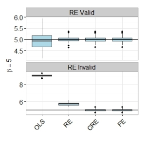
The graph below shows the importance of using panel methods over pooled OLS. It shows boxplots of the 100 simulated estimates. Even when the random effects assumption is violated, the random effects estimator (RE) is far superior to simple pooled OLS. Both the CRE and FE estimators perform well. Both have lowest root mean square errors, even though the model satisfies the random effects assumption. Please see my R code below.

# clear ws
rm(list=ls())

# load packages
library(lme4)
library(plyr)
library(lfe)
library(reshape)
library(ggplot2)
# from this:

### set number of individuals
n = 200
# time periods
t = 5

### model is: y=beta0_{i} +beta1*x_{it} + e_{it}
### average intercept and slope
beta0 = 1.0
beta1 = 5.0

### set loop reps
loop = 100
### results to be entered
results1 = matrix(NA, nrow=loop, ncol=4)
results2 = matrix(NA, nrow=loop, ncol=4)

for(i in 1:loop){
  # basic data structure
  data = data.frame(t = rep(1:t,n),
                    n = sort(rep(1:n,t)))
  # random effect/intercept to add to each 
  rand = data.frame(n = 1:n,
                    a = rnorm(n,0,3))
  data = join(data, rand, match="first")
  # random error
  data$u = rnorm(nrow(data), 0, 1)
  # regressor x
  data$x = runif(nrow(data), 0, 1)
  # outcome y
  data$y = beta0 + beta1*data$x + data$a + data$u  
  # make factor for i-units
  data$n = as.character(data$n)
  # group i mean's for correlated random effects
  data$xn = ave(data$x, data$n, FUN=mean)
  # pooled OLS
  a1 = lm(y ~ x, data)
  # random effects
  a2 = lmer(y ~ x + (1|n), data)
  # correlated random effects
  a3 = lmer(y ~ x + xn + (1|n), data)
  # fixed effects
  a4 = felm(y ~ x | n, data)
  
  # gather results
  results1[i,] = c(coef(a1)[2],
                  coef(a2)$n[1,2],
                  coef(a3)$n[1,2],
                  coef(a4)[1])
  ### now let random effects assumption be false
  ### ie E[xa]!=0
  data$x = runif(nrow(data), 0, 1) + 0.2*data$a
  # the below is like above
  data$y = beta0 + beta1*data$x + data$a + data$u  
  data$n = as.character(data$n)
  data$xn = ave(data$x, data$n, FUN=mean)
  a1 = lm(y ~ x, data)
  a2 = lmer(y ~ x + (1|n), data)
  a3 = lmer(y ~ x + xn + (1|n), data)
  a4 = felm(y ~ x | n, data)
  
  results2[i,] = c(coef(a1)[2],
                  coef(a2)$n[1,2],
                  coef(a3)$n[1,2],
                  coef(a4)[1])  
}
# calculate rmse
apply(results1, 2, function(x) sqrt(mean((x-5)^2)))
apply(results2, 2, function(x) sqrt(mean((x-5)^2)))

# shape data and do ggplot
model.names = data.frame(X2 = c("1","2","3","4"),
                         estimator = c("OLS","RE","CRE","FE"))
res1 = melt(results1)
res1 = join(res1, model.names, match="first")
res2 = melt(results2)
res2 = join(res2, model.names, match="first")

res1$split = "RE Valid"
res2$split = "RE Invalid"
res1 = rbind(res1, res2)

res1$split = factor(res1$split, levels =  c("RE Valid", "RE Invalid"))
res1$estimator = factor(res1$estimator, levels =  c("OLS","RE","CRE","FE"))

number_ticks = function(n) {function(limits) pretty(limits, n)}

ggplot(res1, aes(estimator, value)) + 
  geom_boxplot(fill="lightblue") +
  #coord_flip() +
  facet_wrap( ~ split, nrow = 2, scales = "free_y") +
  geom_hline(yintercept = 5) +
  scale_x_discrete('') + 
  scale_y_continuous(bquote(beta==5), breaks=number_ticks(3)) + 
  theme_bw() + 
  theme(axis.text=element_text(size=16),
        axis.title=element_text(size=16),
        legend.title = element_blank(),
        legend.text = element_text(size=16),
        strip.text.x = element_text(size = 16),
        axis.text.x = element_text(angle = 45, hjust = 1))
ggsave("remc.pdf", width=8, height=6)

How Predictable is the English Premier League?

The reason why football is so exciting is uncertainty. The outcome of any match or league is unknown, and you get to watch the action unfold without knowing what’s going to happen. Watching matches where you know the score is never exciting.

This weekend the English Premier League season will conclude with little fanfare. Bar one relegation place, the league positions have already been determined. In fact, these positions were, for the most part, decided weeks ago. The element of uncertainty seems to have been reduced this season.

With this in mind, I wanted to look at uncertainty over the long run in English football. To do this used the data provided by http://www.football-data.co.uk/ and analyzed these with R. These data consist of 34,740 matches played in the top 5 divisions of English football between 2000 and 2015, containing information about both the result and the odds offered by bookies on this result.

To measure the uncertainty of any given match I used the following strategy. First, I averaged across all bookies’ odds for the three possible events: home win, draw, and away win. Next I mapped these aggregated odds into probabilities by inverting each of the odds and then dividing by the summed inverted odds. This takes care of the over round that helps bookies to make a profit. For example, if the odds were 2.1/1 that an event happens and 2.1/1 that it doesn’t then the probability of the event occurring is:

(1/2.1)/ (1/2.1 + (1/2.1)) = 0.4761905/(0.4761905+0.4761905) = 0.5.

Finally, to measure the uncertainty of each match, I subtract the probability that the event occurred from 1, to calculate a “residual” score. Imagine a home win occurs. The “residual” in this case will be 1-P(home win). If P(home win)=1, then there is no uncertainty, and this uncertainty score will be zero. Since there are 3 outcomes, we would expect an uncertainty measure to be bounded between 0 (no uncertainty) and 0.67 (pure uncertainty) where we get 1 out of 3right by just guessing.

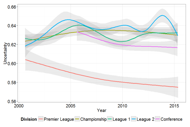
After importing these data into R and calculating the uncertainty measure, I looked at this uncertainty measure over time. The plot in the above shows fitted smoothed trend lines of uncertainty, stratified by division. These trends are striking. Going by this graph, the Premier League has gotten more predictable over the analysis period. In 2000, the uncertainty measure was around 0.605. Given that we expect this measure to be bound between 0 (complete certainty) and 0.67 (completely random), this tell us that the average league game was very unpredictable. Over time, however, this measure has decreased by about 5%, which does not seem like much. Despite, the somewhat unexciting end to the 2014/15 season, the outcome of the average game is still not very predictable.

Noticeably, in lower league games there is even greater uncertainty. In fact, the average uncertainty measure of League 2 games approached a value of 0.65 in 2014. This indicates that the average League 2 game is about as unpredictable as playing rock-paper-scissors. Interestingly, and unlike the Premier League, there does not appear to be any discernible change over time. The games are just as unpredictable now as they were in 2000. Please see my R code below.

# clear
rm(list=ls())

# libraries
library(ggplot2)

# what are urls

years = c(rep("0001",4), rep("0102",4), rep("0203",4), rep("0405",4),
          rep("0506",5), rep("0607",5), rep("0708",5), rep("0809",5),
          rep("0910",5), rep("1011",5), rep("1112",5), rep("1213",5),
          rep("1314",5), rep("1415",5))
divis = c(rep(c("E0","E1","E2","E3"),4), rep(c("E0","E1","E2","E3","EC"),10))

urls = paste(years, divis, sep="/")
urls = paste("http://www.football-data.co.uk/mmz4281", urls, sep="/")


odds = c("B365H","B365D","B365A",
         "BSH","BSD","BSA",
         "BWH","BWD","BWA",
         "GBH","GBD","GBA",
         "IWH","IWD","IWA",
         "LBH","LBD","LBA",
         "PSH","PSD","PSA",
         "SOH","SOD","SOA",
         "SBH","SBD","SBA",
         "SJH","SJD","SJA",
         "SYH","SYD","SYA",
         "VCH","VCD","VCA",
         "WHH","WHD","WHA")
home = odds[seq(1,length(odds),3)]
draw = odds[seq(2,length(odds),3)]
away = odds[seq(3,length(odds),3)]

# load all data in a loop
full.data = NULL
for(i in 1:length(urls)){
  temp = read.csv(urls[i])
  # calculate average odds
  temp$homeodds = apply(temp[,names(temp) %in% home], 1, function(x) mean(x,na.rm=T))
  temp$drawodds = apply(temp[,names(temp) %in% draw], 1, function(x) mean(x,na.rm=T))
  temp$awayodds = apply(temp[,names(temp) %in% away], 1, function(x) mean(x,na.rm=T))
  temp = temp[,c("Div","Date","FTHG","FTAG","FTR","homeodds","drawodds","awayodds")]
  full.data = rbind(full.data, temp)
}

full.data$homewin = ifelse(full.data$FTR=="H", 1, 0)
full.data$draw = ifelse(full.data$FTR=="D", 1, 0)
full.data$awaywin = ifelse(full.data$FTR=="A", 1, 0)

# convert to probs with overrind
full.data$homeprob = (1/full.data$homeodds)/(1/full.data$homeodds+1/full.data$drawodds+1/full.data$awayodds)
full.data$drawprob = (1/full.data$drawodds)/(1/full.data$homeodds+1/full.data$drawodds+1/full.data$awayodds)
full.data$awayprob = (1/full.data$awayodds)/(1/full.data$homeodds+1/full.data$drawodds+1/full.data$awayodds)

# bookie residual
full.data$bookieres = 1-full.data$homeprob
full.data$bookieres[full.data$FTR=="D"] = 1-full.data$drawprob[full.data$FTR=="D"]
full.data$bookieres[full.data$FTR=="A"] = 1-full.data$awayprob[full.data$FTR=="A"]

# now plot over time
full.data$time = ifelse(nchar(as.character(full.data$Date))==8, 
                         as.Date(full.data$Date,format='%d/%m/%y'),
                         as.Date(full.data$Date,format='%d/%m/%Y'))
full.data$date = as.Date(full.data$time, origin = "1970-01-01") 

full.data$Division = "Premier League" 
full.data$Division[full.data$Div=="E1"] = "Championship" 
full.data$Division[full.data$Div=="E2"] = "League 1" 
full.data$Division[full.data$Div=="E3"] = "League 2" 
full.data$Division[full.data$Div=="EC"] = "Conference" 

full.data$Division = factor(full.data$Division, levels = c("Premier League", "Championship", "League 1",
                                                           "League 2","Conference"))

ggplot(full.data, aes(date, bookieres, colour=Division)) +
  stat_smooth(size = 1.25, alpha = 0.2) +
  labs(x = "Year", y = "Uncertainty") + 
  theme_bw() +
  theme(legend.position="bottom") +
  theme(axis.text=element_text(size=20),
        axis.title=element_text(size=20),
        legend.title = element_text(size=20),
        legend.text = element_text(size=20))

Coal and the Conservatives

Interesting election results in the UK over the weekend, where the Conservatives romped to victory. This was despite a widespread consensus that neither the Conservative or Labour party would get a majority. This was a triumph for uncertainty and random error over the deterministic, as none of the statistical forecasts appeared to deem such a decisive victory probable. The UK election is a lot harder to model, for numerous reasons, when compared to the US.

This means that a lot of pollsters and political forecasters will have to go back to the drawing board and re-evaluate their methods. Obviously, the models used to forecast the 2015 election could not handle the dynamics of the British electorate. However, there is a high degree of persistence within electuary constituencies. Let’s explore this persistence by looking at the relationship between coal and % Conservative (Tory) votes.

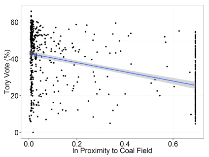
Following a tweet by Vaughan Roderick and using the methodology of Fernihough and O’Rourke (2014), I matched each of the constituencies to Britain’s coalfields creating a “proximity to coal” measure. What the plot below shows is striking. Being located on or in close proximity to a coal field reduces the tory vote share by about 20%. When we control (linearly) for latitude and longitude coordinates, this association decreases in strength, but not by much. For me, this plot highlights a long-standing relationship between Britain’s industrial revolution, the urban working class, and labour/union movement. What I find interesting is that this relationship has persisted despite de-industrialization and the movement away from large-scale manufacturing industry.

> summary(lm(tory~coal,city))

Call:
lm(formula = tory ~ coal, data = city)

Residuals:
    Min      1Q  Median      3Q     Max 
-42.507 -10.494   2.242  10.781  29.074 

Coefficients:
            Estimate Std. Error t value Pr(>|t|)    
(Intercept)  42.9492     0.7459   57.58   <2e-16 ***
coal        -24.9704     1.8887  -13.22   <2e-16 ***
---
Signif. codes:  0 ‘***’ 0.001 ‘**’ 0.01 ‘*’ 0.05 ‘.’ 0.1 ‘ ’ 1

Residual standard error: 14.36 on 630 degrees of freedom
Multiple R-squared:  0.2172,	Adjusted R-squared:  0.216 
F-statistic: 174.8 on 1 and 630 DF,  p-value: < 2.2e-16

# robust to lat-long?
> summary(lm(tory~coal+longitude+latitude,city))

Call:
lm(formula = tory ~ coal + longitude + latitude, data = city)

Residuals:
    Min      1Q  Median      3Q     Max 
-44.495  -8.269   1.485   9.316  28.911 

Coefficients:
            Estimate Std. Error t value Pr(>|t|)    
(Intercept) 246.4355    18.9430  13.009  < 2e-16 ***
coal        -15.1616     1.8697  -8.109 2.68e-15 ***
longitude     1.4023     0.4015   3.493 0.000512 ***
latitude     -3.8621     0.3651 -10.578  < 2e-16 ***
---
Signif. codes:  0 ‘***’ 0.001 ‘**’ 0.01 ‘*’ 0.05 ‘.’ 0.1 ‘ ’ 1

Residual standard error: 12.76 on 628 degrees of freedom
Multiple R-squared:  0.3838,	Adjusted R-squared:  0.3809 
F-statistic: 130.4 on 3 and 628 DF,  p-value: < 2.2e-16

Brazil’s Host Advantage

If history can tell us anything about the World Cup, it’s that the host nation has an advantage of all other teams. Evidence of this was presented last night as the referee in the Brazil-Croatia match unjustly ruled in Brazil’s favour on several occasions. But what it is the statistical evidence of a host advantage?

To look at this, I downloaded these data from the Guardian’s website. With these, I ran a very simple probit model that regressed the probability of winning the world cup on whether the country was the host and also if the county was not the host but located in the same continent (I merge North and South America for this exercise). Obviously, this is quite a basic analysis, so I hope to build on these data as the tournament progresses and maybe and the 2010 data, and look at more sophisticated models.

> probitmfx(formula=winners ~ continent + hosts, data=wc)
Call:
probitmfx(formula = winners ~ continent + hosts, data = wc)

Marginal Effects:
             dF/dx Std. Err.      z   P>|z|   
continent 0.064425  0.027018 2.3845 0.01710 * 
hosts     0.315378  0.121175 2.6027 0.00925 **
---
Signif. codes:  0 ‘***’ 0.001 ‘**’ 0.01 ‘*’ 0.05 ‘.’ 0.1 ‘ ’ 1

dF/dx is for discrete change for the following variables:

[1] "continent" "hosts"   

The results are as we would expect. I am using the excellent mfx package to interpret the probit coefficients. Being the host nation increases the probability of being victorious by nearly 32%. So, going by historical trends, Brazil have a huge advantage for this world cup. If we look at countries in the same continent (think Argentina for this world cup) we see that there is a small advantage here, just over 6%.

Whether these results are robust to additional control variables and in the inclusion of fixed effects alongside heterogeneous time-varying effects is something I hope to probe.

The ivlewbel Package. A new way to Tackle Endogenous Regressor Models.

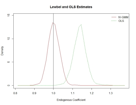
In April 2012, I wrote this blog post demonstrating an approach proposed in Lewbel (2012) that identifies endogenous regressor coefficients in a linear triangular system. Now I am happy to announce the release of the ivlewbel package, which contains a function through which Lewbel’s method can be applied in R. This package is now available to download on the CRAN.

Please see the example from the previous blog post replicated in the below. Additionally, it would be very helpful if people could comment on bugs and additional features they would like to add to the package. My contact details are in the about section of the blog.

library(ivlewbel)

beta1 <- beta2 <- NULL
for(k in 1:500){
  #generate data (including intercept)
  x1 <- rnorm(1000,0,1)
  x2 <- rnorm(1000,0,1)
  u <- rnorm(1000,0,1)
  s1 <- rnorm(1000,0,1)
  s2 <- rnorm(1000,0,1)
  ov <- rnorm(1000,0,1)
  e1 <- u + exp(x1)*s1 + exp(x2)*s1
  e2 <- u + exp(-x1)*s2 + exp(-x2)*s2
  y1 <- 1 + x1 + x2 + ov + e2 
  y2 <- 1 + x1 + x2 + y1 + 2*ov + e1
  x3 <- rep(1,1000)
  dat <- data.frame(y1,y2,x3,x1,x2)
  
  #record ols estimate
  beta1 <- c(beta1,coef(lm(y2~x1+x2+y1))[4])
  #init values for iv-gmm
  beta2 <- c(beta2,lewbel(formula = y2 ~ y1 | x1 + x2 | x1 + x2, data = dat)$coef.est[1,1])
}

library(sm)
d <- data.frame(rbind(cbind(beta1,"OLS"),cbind(beta2,"IV-GMM")))
d$beta1 <- as.numeric(as.character(d$beta1))
sm.density.compare(d$beta1, d$V2,xlab=("Endogenous Coefficient"))
title("Lewbel and OLS Estimates")
legend("topright", levels(d$V2),lty=c(1,2,3),col=c(2,3,4),bty="n")
abline(v=1)

IV Estimates via GMM with Clustering in R

In econometrics, generalized method of moments (GMM) is one estimation methodology that can be used to calculate instrumental variable (IV) estimates. Performing this calculation in R, for a linear IV model, is trivial. One simply uses the gmm() function in the excellent gmm package like an lm() or ivreg() function. The gmm() function will estimate the regression and return model coefficients and their standard errors. An interesting feature of this function, and GMM estimators in general, is that they contain a test of over-identification, often dubbed Hansen’s J-test, as an inherent feature. Therefore, in cases where the researcher is lucky enough to have more instruments than endogenous regressors, they should examine this over-identification test post-estimation.

While the gmm() function in R is very flexible, it does not (yet) allow the user to estimate a GMM model that produces standard errors and an over-identification test that is corrected for clustering. Thankfully, the gmm() function is flexible enough to allow for a simple hack that works around this small shortcoming. For this, I have created a function called gmmcl(), and you can find the code below. This is a function for a basic linear IV model. This code uses the gmm() function to estimate both steps in a two-step feasible GMM procedure. The key to allowing for clustering is to adjust the weights matrix after the second step. Interested readers can find more technical details regarding this approach here. After defining the function, I show a simple application in the code below.

gmmcl = function(formula1, formula2, data, cluster){
  library(plyr) ; library(gmm)
  # create data.frame
  data$id1 = 1:dim(data)[1]
  formula3 = paste(as.character(formula1)[3],"id1", sep=" + ")
  formula4 = paste(as.character(formula1)[2], formula3, sep=" ~ ")
  formula4 = as.formula(formula4)
  formula5 = paste(as.character(formula2)[2],"id1", sep=" + ")
  formula6 = paste(" ~ ", formula5, sep=" ")
  formula6 = as.formula(formula6)
  frame1 = model.frame(formula4, data)
  frame2 = model.frame(formula6, data)
  dat1 = join(data, frame1, type="inner", match="first")
  dat2 = join(dat1, frame2, type="inner", match="first")
  
  # matrix of instruments
  Z1 = model.matrix(formula2, dat2)
  
  # step 1
  gmm1 = gmm(formula1, formula2, data = dat2, 
             vcov="TrueFixed", weightsMatrix = diag(dim(Z1)[2]))
  
  # clustering weight matrix
  cluster = factor(dat2[,cluster])
  u = residuals(gmm1)
  estfun = sweep(Z1, MARGIN=1, u,'*')
  u = apply(estfun, 2, function(x) tapply(x, cluster, sum))  
  S = 1/(length(residuals(gmm1)))*crossprod(u)
  
  # step 2
  gmm2 = gmm(formula1, formula2, data=dat2, 
             vcov="TrueFixed", weightsMatrix = solve(S))
  return(gmm2)
}

# generate data.frame
n = 100
z1 = rnorm(n)
z2 = rnorm(n)
x1 = z1 + z2 + rnorm(n)
y1 = x1 + rnorm(n)
id = 1:n

data = data.frame(z1 = c(z1, z1), z2 = c(z2, z2), x1 = c(x1, x1),
                  y1 = c(y1, y1), id = c(id, id))

summary(gmmcl(y1 ~ x1, ~ z1 + z2, data = data, cluster = "id"))

Within Group Index in R

There are many occasions in my research when I want to create a within group index for a data frame. For example, with demographic data for siblings one might want to create a birth order index.

The below illustrates a simple example of how one can create such an index in R.

set.seed(123)
# two families/groups 1 and 2
# with random ages
data = data.frame(group = c(rep(1,5),rep(2,5)), age = rpois(10,10))

# birth order
# use rank function with negative age for descending order
data$bo = unlist(by(data, data$group, 
                    function(x) rank(-x$age, ties.method = "first")))

Detecting Weak Instruments in R

Weak Instruments

Any instrumental variables (IV) estimator relies on two key assumptions in order to identify causal effects:

1. That the excluded instrument or instruments only effect the dependent variable through their effect on the endogenous explanatory variable or variables (the exclusion restriction),
2. That the correlation between the excluded instruments and the endogenous explanatory variables is strong enough to permit identification.

The first assumption is difficult or impossible to test, and shear belief plays a big part in what can be perceived to be a good IV. An interesting paper was published last year in the Review of Economics and Statistics by Conley, Hansen, and Rossi (2012), wherein the authors provide a Bayesian framework that permits researchers to explore the consequences of relaxing exclusion restrictions in a linear IV estimator. It will be interesting to watch research on this topic expand in the coming years.

Fortunately, it is possible to quantitatively measure the strength of the relationship between the IVs and the endogenous variables. The so-called weak IV problem was underlined in paper by Bound, Jaeger, and Baker (1995). When the relationship between the IVs and the endogenous variable is not sufficiently strong, IV estimators do not correctly identify causal effects.

The Bound, Jaeger, and Baker paper represented a very important contribution to the econometrics literature. As a result of this paper, empirical studies that use IV almost always report some measure of the instrument strength. A secondary result of this paper was the establishment of a literature that evaluates different methods of testing for weak IVs. Staiger and Stock (1997) furthered this research agenda, formalizing the relevant asymptotic theory and recommending the now ubiquitous “rule-of-thumb” measure: a first-stage partial-F test of less than 10 indicates the presence of weak instruments.

In the code below, I have illustrated how one can perform these partial F-tests in R. The importance of clustered standard errors has been highlighted on this blog before, so I also show how the partial F-test can be performed in the presence of clustering (and heteroskedasticity too). To obtain the clustered variance-covariance matrix, I have adapted some code kindly provided by Ian Gow. For completeness, I have displayed the clustering function at the end of the blog post.

# load packages
library(AER) ; library(foreign) ; library(mvtnorm)
# clear workspace and set seed
rm(list=ls())
set.seed(100)

# number of observations
n = 1000
# simple triangular model:
# y2 = b1 + b2x1 + b3y1 + e
# y1 = a1 + a2x1 + a3z1 + u
# error terms (u and e) correlate 
Sigma = matrix(c(1,0.5,0.5,1),2,2)
ue = rmvnorm(n, rep(0,2), Sigma)
# iv variable
z1 = rnorm(n)
x1 = rnorm(n)
y1 = 0.3 + 0.8*x1 - 0.5*z1 + ue[,1]
y2 = -0.9 + 0.2*x1 + 0.75*y1 +ue[,2]
# create data
dat = data.frame(z1, x1, y1, y2)

# biased OLS
lm(y2 ~ x1 + y1, data=dat)
# IV (2SLS)
ivreg(y2 ~ x1 + y1 | x1 + z1, data=dat)

# do regressions for partial F-tests
# first-stage:
fs = lm(y1 ~ x1 + z1, data = dat)
# null first-stage (i.e. exclude IVs):
fn = lm(y1 ~ x1, data = dat)

# simple F-test
waldtest(fs, fn)$F[2]
# F-test robust to heteroskedasticity
waldtest(fs, fn, vcov = vcovHC(fs, type="HC0"))$F[2]

####################################################
# now lets get some F-tests robust to clustering

# generate cluster variable
dat$cluster = 1:n
# repeat dataset 10 times to artificially reduce standard errors
dat = dat[rep(seq_len(nrow(dat)), 10), ]

# re-run first-stage regressions
fs = lm(y1 ~ x1 + z1, data = dat)
fn = lm(y1 ~ x1, data = dat)

# simple F-test
waldtest(fs, fn)$F[2]
# ~ 10 times higher!
# F-test robust to clustering
waldtest(fs, fn, vcov = clusterVCV(dat, fs, cluster1="cluster"))$F[2]
# ~ 10 times lower than above (good)

Further “rule-of-thumb” measures are provided in a paper by Stock and Yogo (2005) and it should be noted that whole battery of weak-IV tests exist (for example, see the Kleinberg-Paap rank Wald F-statistic and Anderson-Rubin Wald test) and one should perform these tests if the presence of weak instruments represents a serious concern. 

# R function adapted from Ian Gows' webpage:
# http://www.people.hbs.edu/igow/GOT/Code/cluster2.R.html.
clusterVCV <- function(data, fm, cluster1, cluster2=NULL) {
  
  require(sandwich)
  require(lmtest)
  
  # Calculation shared by covariance estimates
  est.fun <- estfun(fm)
  inc.obs <- complete.cases(data[,names(fm$model)])
  
  # Shared data for degrees-of-freedom corrections
  N  <- dim(fm$model)[1]
  NROW <- NROW(est.fun)
  K  <- fm$rank
  
  # Calculate the sandwich covariance estimate
  cov <- function(cluster) {
    cluster <- factor(cluster)
    
    # Calculate the "meat" of the sandwich estimators
    u <- apply(est.fun, 2, function(x) tapply(x, cluster, sum))
    meat <- crossprod(u)/N
    
    # Calculations for degrees-of-freedom corrections, followed 
    # by calculation of the variance-covariance estimate.
    # NOTE: NROW/N is a kluge to address the fact that sandwich uses the
    # wrong number of rows (includes rows omitted from the regression).
    M <- length(levels(cluster))
    dfc <- M/(M-1) * (N-1)/(N-K)
    dfc * NROW/N * sandwich(fm, meat=meat)
  }
  
  # Calculate the covariance matrix estimate for the first cluster.
  cluster1 <- data[inc.obs,cluster1]
  cov1  <- cov(cluster1)
  
  if(is.null(cluster2)) {
    # If only one cluster supplied, return single cluster
    # results
    return(cov1)
  } else {
    # Otherwise do the calculations for the second cluster
    # and the "intersection" cluster.
    cluster2 <- data[inc.obs,cluster2]
    cluster12 <- paste(cluster1,cluster2, sep="")
    
    # Calculate the covariance matrices for cluster2, the "intersection"
    # cluster, then then put all the pieces together.
    cov2   <- cov(cluster2)
    cov12  <- cov(cluster12)
    covMCL <- (cov1 + cov2 - cov12)
    
    # Return the output of coeftest using two-way cluster-robust
    # standard errors.
    return(covMCL)
  }
}